Natural Language Processing

Useful links for NLP and processing text input for intent:

https://dialogflow.com/    (was api.ai)

https://github.com/cjhutto/vaderSentiment    << vader sentiment for sentiment analysis

RASA NLU - https://github.com/RasaHQ/rasa_nlu


Building a recommender system using Python:

https://www.lynda.com/Python-tutorials/Introduction-Python-Recommendation-Systems-Machine-Learning/


Building a skill with AWS Lambda
https://moduscreate.com/build-an-alexa-skill-with-python-and-aws-lambda/


SQuAD - Standford QA dataset
https://rajpurkar.github.io/SQuAD-explorer/


Facebook babi project:  https://research.fb.com/downloads/babi/


http://www.geo.uzh.ch/~rsp/semGeoSoc/  : transparent use of semantics embedded in geosocial and other data for helping mobile users in their decision-making 

Natural Language Processing - link to intro article

The original article can be found here:
https://www.kdnuggets.com/2017/02/natural-language-processing-key-terms-explained.html


Article by  Matthew Mayo, KDnuggets. 

1. Natural Language Processing (NLP)

Natural language processing (NLP) concerns itself with the interaction between natural human languages and computing devices. NLP is a major aspect of computational linguistics, and also falls within the realms of computer science and artificial intelligence.

2. Tokenization

Tokenization is, generally, an early step in the NLP process, a step which splits longer strings of text into smaller pieces, or tokens. Larger chunks of text can be tokenized into sentences, sentences can be tokenized into words, etc. Further processing is generally performed after a piece of text has been appropriately tokenized.

3. Normalization

Before further processing, text needs to be normalized. Normalization generally refers to a series of related tasks meant to put all text on a level playing field: converting all text to the same case (upper or lower), removing punctuation, expanding contractions, converting numbers to their word equivalents, and so on. Normalization puts all words on equal footing, and allows processing to proceed uniformly.

4. Stemming

Stemming is the process of eliminating affixes (suffixed, prefixes, infixes, circumfixes) from a word in order to obtain a word stem.

running → run

5. Lemmatization

Lemmatization is related to stemming, differing in that lemmatization is able to capture canonical forms based on a word's lemma.

For example, stemming the word "better" would fail to return its citation form (another word for lemma); however, lemmatization would result in the following:

better → good

It should be easy to see why the implementation of a stemmer would be the less difficult feat of the two.

6. Corpus

In linguistics and NLP, corpus (literally Latin for body) refers to a collection of texts. Such collections may be formed of a single language of texts, or can span multiple languages -- there are numerous reasons for which multilingual corpora (the plural of corpus) may be useful. Corpora may also consist of themed texts (historical, Biblical, etc.). Corpora are generally solely used for statistical linguistic analysis and hypothesis testing.

7. Stop Words

Stop words are those words which are filtered out before further processing of text, since these words contribute little to overall meaning, given that they are generally the most common words in a language. For instance, "the," "and," and "a," while all required words in a particular passage, don't generally contribute greatly to one's understanding of content. As a simple example, the following panagram is just as legible if the stop words are removed:

The quick brown fox jumps over the lazy dog.

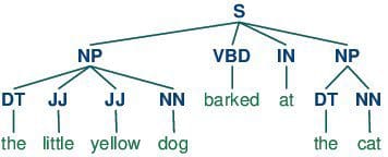
8. Parts-of-speech (POS) Tagging

POS tagging consists of assigning a category tag to the tokenized parts of a sentence. The most popular POS tagging would be identifying words as nouns, verbs, adjectives, etc.

9. Statistical Language Modeling

Statistical Language Modeling is the process of building a statistical language model which is meant to provide an estimate of a natural language. For a sequence of input words, the model would assign a probability to the entire sequence, which contributes to the estimated likelihood of various possible sequences. This can be especially useful for NLP applications which generate text.

10. Bag of Words

Bag of words is a particular representation model used to simplify the contents of a selection of text. The bag of words model omits grammar and word order, but is interested in the number of occurrences of words within the text. The ultimate representation of the text selection is that of a bag of words (bag referring to the set theory concept of multisets, which differ from simple sets).

Actual storage mechanisms for the bag of words representation can vary, but the following is a simple example using a dictionary for intuitiveness. Sample text:

"Well, well, well," said John.

"There, there," said James. "There, there."

The resulting bag of words representation as a dictionary:

   {
      'well': 3,
      'said': 2,
      'john': 1,
      'there': 4,
      'james': 1
   }

11. n-grams

n-grams is another representation model for simplifying text selection contents. As opposed to the orderless representation of bag of words, n-grams modeling is interested in preserving contiguous sequences of N items from the text selection.

An example of trigram (3-gram) model of the second sentence of the above example ("There, there," said James. "There, there.") appears as a list representation below:

   [
      "there there said",
      "there said james",
      "said james there",
      "james there there",
   ]

12. Regular Expressions

Regular expressions, often abbreviated regexp or regexp, are a tried and true method of concisely describing patterns of text. A regular expression is represented as a special text string itself, and is meant for developing search patterns on selections of text. Regular expressions can be thought of as an expanded set of rules beyond the wildcard characters of ? and *. Though often cited as frustrating to learn, regular expressions are incredibly powerful text searching tools.

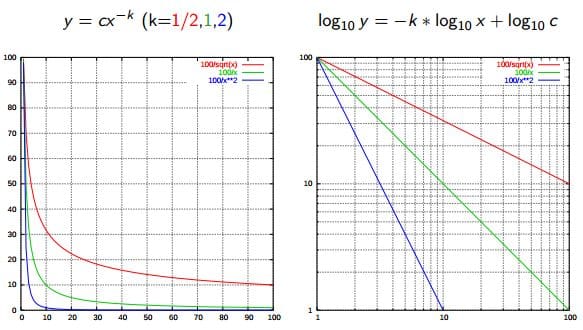
13. Zipf's Law

Zipf's Law is used to describe the relationship between word frequencies in document collections. If a document collection's words are ordered by frequency, and y is used to describe the number of times that the xth word appears, Zipf's observation is concisely captured as y = cx^-1/2 (item frequency is inversely proportional to item rank). More generally, Wikipedia says:

Zipf's law states that given some corpus of natural language utterances, the frequency of any word is inversely proportional to its rank in the frequency table. Thus the most frequent word will occur approximately twice as often as the second most frequent word, three times as often as the third most frequent word, etc.

14. Similarity Measures

There are numerous similarity measures which can be applied to NLP. What are we measuring the similarity of? Generally, strings.

• Levenshtein - the number of characters that must be deleted, inserted, or substituted in order to make a pair of strings equal
• Jaccard - the measure of overlap between 2 sets; in the case of NLP, generally, documents are sets of words
• Smith Waterman - similar to Levenshtein, but with costs assigned to substitution, insertion, and deletion

15. Syntactic Analysis

Also referred to as parsing, syntactic analysis is the task of analyzing strings as symbols, and ensuring their conformance to a established set of grammatical rules. This step must, out of necessity, come before any further analysis which attempts to extract insight from text -- semantic, sentiment, etc. -- treating it as something beyond symbols.

16. Semantic Analysis

Also known as meaning generation, semantic analysis is interested in determining the meaning of text selections (either character or word sequences). After an input selection of text is read and parsed (analyzed syntactically), the text selection can then be interpreted for meaning. Simply put, syntactic analysis is concerned with what words a text selection was made up of, while semantic analysis wants to know what the collection of words actually means. The topic of semantic analysis is both broad and deep, with a wide variety of tools and techniques at the researcher's disposal.

17. Sentiment Analysis

Sentiment analysis is the process of evaluating and determining the sentiment captured in a selection of text, with sentiment defined as feeling or emotion. This sentiment can be simply positive (happy), negative (sad or angry), or neutral, or can be some more precise measurement along a scale, with neutral in the middle, and positive and negative increasing in either direction.

18. Information Retrieval

Information retrieval is the process of accessing and retrieving the most appropriate information from text based on a particular query, using context-based indexing or metadata. One of the most famous examples of information retrieval would be Google Search.

Linux Disk Tools

Useful commands when adding a new HDD to a Linux server


sudo gparted  
  >>partition disk etc


sudo gnome-disks
>> configure mount location

Geographic Weighted Regression

Good video   http://www.youtube.com/watch?v=plfCMZhROeQ

Regression has explanatory variables (also known as independant variables) and they have strengths (coefficients)

These inputs result in our dependant variable

+ or - for the coefficients

(if Beta goes up and the number of incidents goes down then a NEGative relationship)

_______________________________________________________________

Confusion Matrix for Machine Learning or Image Classifications

Great guide here: http://spatial-analyst.net/ILWIS/htm/ilwismen/confusion_matrix.htm

Copied below for archiving (all credit to original authors).

========

To assess the accuracy of an image classification, it is common practice to create a confusion matrix. In a confusion matrix, your classification results are compared to additional ground truth information. The strength of a confusion matrix is that it identifies the nature of the classification errors, as well as their quantities.

Tip: The output cross table of a Cross operation on two maps which use a class or ID domain, can also be shown in matrix form. For more information, refer to Cross : functionality.

Preparation:

• Create a raster map which contains additional ground truth information (such a map is also known as the test set). It is strongly advised that the test set raster map does not contain the same pixels as the sample set raster map from the training phase.
• Furthermore, the output raster map of the image classification is required.
• Then, perform a Cross with the ground truth map and the classified map to obtain a cross table.
• Open the cross table in a table window, and choose Confusion matrix from the View menu in the table window.

The details of these steps are described in How to calculate a confusion matrix.

Dialog box options:

First column:	Select the column with the same name as the ground truth map (or test set).
Second column:	Select the column with the same name as the output map of the Classify operation.
Frequency:	Select the NPix column.

The confusion matrix appears in a secondary window.

Note:

• If in the dialog box, you choose the ground truth map for the first column, and the classification results for the second column (i.e. the same as shown above), then the ground truth can be found in the rows of the confusion matrix, and the classification results will appear in the columns. You can read the explanation below without further changes.
• However, if in the dialog box, you choose the classification results as the first column, and the ground truth map for the second column (i.e. reverse as shown above), then the classification results can be found in the rows in the confusion matrix, and the ground truth will appear in the columns. You will then have to read 'columns' instead of 'rows', and 'rows' instead of 'columns' in the remainder of this topic. Furthermore you should read ACC (accuracy) instead of REL (reliability) and vice versa.

Interpretation of a confusion matrix:

Consider the following example of a confusion matrix:

  

CLASSIFICATION RESULTS

		forest	bush	crop	urban	bare	water	unclass	ACC
GROUND	forest	440	40	0	0	30	10	10	0.83
TRUTH	bush	20	220	0	0	40	10	20	0.71
	crop	10	10	210	10	50	10	60	0.58
	urban	20	0	20	240	100	10	40	0.56
	bare	0	0	10	10	230	0	10	0.88
	water	0	20	0	0	0	240	10	0.89
	REL	0.90	0.76	0.88	0.92	0.51	0.86

  

Average accuracy	=	74.25%
Average reliability	=	80.38%
Overall accuracy	=	73.15%

In the example above:

• unclass represents the Unclassified column,
• ACC represents the Accuracy column,
• REL represents the Reliability column.

Explanation:

• Rows correspond to classes in the ground truth map (or test set).
• Columns correspond to classes in the classification result.
• The diagonal elements in the matrix represent the number of correctly classified pixels of each class, i.e. the number of ground truth pixels with a certain class name that actually obtained the same class name during classification. In the example above, 440 pixels of 'forest' in the test set were correctly classified as 'forest' in the classified image.
• The off-diagonal elements represent misclassified pixels or the classification errors, i.e. the number of ground truth pixels that ended up in another class during classification. In the example above, 40 pixels of 'forest' in the test set were classified as 'bush' in the classified image.
  
  • Off-diagonal row elements represent ground truth pixels of a certain class which were excluded from that class during classification. Such errors are also known as errors of omission or exclusion. For example, 50 ground truth pixels of 'crop' were excluded from the 'crop' class in the classification and ended up in the 'bare' class.
  • Off-diagonal column elements represent ground truth pixels of other classes that were included in a certain classification class. Such errors are also known as errors of commission or inclusion. For example, 100 ground truth pixels of 'urban' were included in the 'bare' class by the classification.
• The figures in column Unclassified represent the ground truth pixels that were found not classified in the classified image.

Accuracy (also known as producer's accuracy): The figures in column Accuracy (ACC) present the accuracy of your classification: it is the fraction of correctly classified pixels with regard to all pixels of that ground truth class. For each class of ground truth pixels (row), the number of correctly classified pixels is divided by the total number of ground truth or test pixels of that class. For example, for the 'forest' class, the accuracy is 440/530 = 0.83 meaning that approximately 83% of the 'forest' ground truth pixels also appear as 'forest' pixels in the classified image.

Reliability (also known as user's accuracy): The figures in row Reliability (REL) present the reliability of classes in the classified image: it is the fraction of correctly classified pixels with regard to all pixels classified as this class in the classified image. For each class in the classified image (column), the number of correctly classified pixels is divided by the total number of pixels which were classified as this class. For example, for the 'forest' class, the reliability is 440/490 = 0.90 meaning that approximately 90% of the 'forest' pixels in the classified image actually represent 'forest' on the ground.

The average accuracy is calculated as the sum of the accuracy figures in column Accuracy divided by the number of classes in the test set.

The average reliability is calculated as the sum of the reliability figures in column Reliability divided by the number of classes in the test set.

The overall accuracy is calculated as the total number of correctly classified pixels (diagonal elements) divided by the total number of test pixels.

From the example above, you can conclude that the test set classes 'crop' and 'urban' were difficult to classify as many of such test set pixels were excluded from the 'crop' and the 'urban' classes, thus the areas of these classes in the classified image are probably underestimated. On the other hand, class 'bare' in the image is not very reliable as many test set pixels of other classes were included in the 'bare' class in the classified image, thus the area of the 'bare' class in the classified image is probably overestimated.

Note:

The results of your confusion matrix highly depend on the selection of ground truth / test set pixels. You may find yourself in a situation of the chicken-egg problem with your sample set, the classification result and your test set. On the one hand, you want to have as many correct sample set pixels as possible so that the classification will be OK; on the other hand, you also need to have an ample number of correct ground truth pixels for the test set to be able to assess the accuracy and reliability of your classification. Using the same data for both the sample set and the test set will produce far too optimistic figures in the confusion matrix. It is mathematically correct to use half of your ground truth data for the sample set and the other half for the test set.

Sony Z5 Compact upgrade to Nougat killed the WiFi Hotspot

How to get it back...  (archive copy held here - all credit &  thanks to original author)

SOURCE

http://www.lukecjdavis.com/fix-internet-tethering-on-lollipop-xperia-z3-plus-other-android-devices/ 

1. Enable developer mode (Go to Settings -> About phone, and press on the build number multiple times until the developer mode is enabled).
2. Click back – you should see a new ‘Developer options’ menu entry. Inside this option enable USB debugging
3. On a computer, install ‘15 seconds ADB Installer’ – available from the XDA Developers forum here. I selected ‘Yes’ for each install option.
4. Connect the phone with a USB cable to the computer, ensuring you press ‘Allow’ to trust your connected computer from the phone
5. Open a command prompt (cmd.exe) and navigate to the ‘adb’ folder directory (C:\adb if you installed system-wide – C:\%UserProfile%\adb if it was installed for the current user only). Type, for example: cd C:\adb\
   
   On Mac:  bash    then      cd /Users/{username}/Library/Android/sdk/platform-tools
                                
6. Start an adb shell by typing the following command: adb shell       (or ./adb shell on Mac)
7. At the adb shell prompt, run this command: settings put global tether_dun_required 0
8. Type exit, then disconnect your phone and reboot

Docker notes

LINUX UBUNTU

install Using Mapserver container https://github.com/srounet/docker-mapserver

To run a new Docker container - mapping the external : internal ports

sudo docker run -d -p HOST_CUSTOM_PORT:80 -v /usr/local/mapserver:/maps --name mapserver mapserver

For example:
 sudo docker run -d -p 81:80 -v /usr/local/mapserver:/maps --name mapserver mapserver


To get to BASH in the container
sudo docker exec -i -t mapserver bash

OR

docker exec -it mapserver sh

To Test it:
http://YOUR_IPADDRESS:PORT/cgi-bin/mapserv


To add a link to your host machine as a resource


Copy files in and out of a docker containedo

docker cp foo.txt mycontainer:/foo.txt
docker cp mycontainer:/foo.txt foo.txt

LIST ALL CONTAINERS RUNNING
sudo docker ps

KILL A RUNNING CONTAINER
sudo docker kill {name of container}


REMOVE CONTAINER
sudo docker rm {name of container}